
This week I wrote code in Julia to create visualizations of the series of chords I wrote about before. I’ll go into the programming process later this post. First, the mathemusical stuff. Let’s have a look at a minor chord, and then I’ll explain what we’re seeing.

This is all based on an article I referenced before, and the concept of a “critical bandwidth of the human ear,” which is well studied. However, my programming is preliminary and rough, so these images are by no means definitive. I hope to refine and improve them in the future, and using a more complete and accurate theory of critical bands.
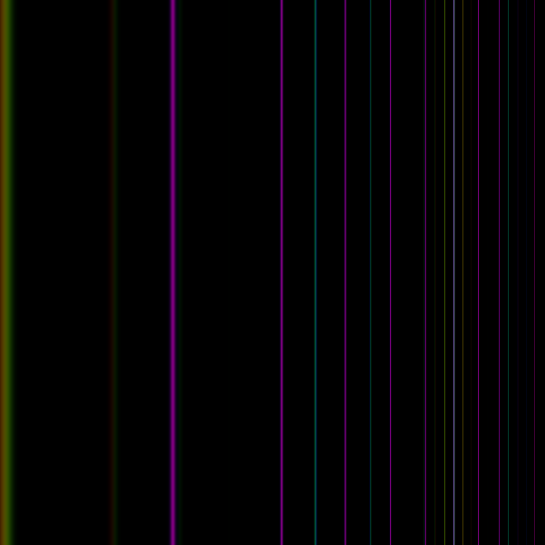
The images each show the overlaps in the harmonic series above a three-note chord. The brightness indicates completeness of overlap and the colour indicates which notes’ series are overlapping: red for the root, green for the variable note M, and blue for the fifth. Therefore a magenta stripe indicates an overlap between the root and fifth, yellow is between the root and M, and cyan is between M and the fifth. A white stripe is where all three overlap, and a dim or murky stripe is where overlap is partial. It should be noted that this is based on my programming, and if I had made the underlying function more or less sensitive, it would change what we define as “partial,” and I will have to do so if I want to refine these. As it stands, the direct overlap between notes two semitones apart is very dim, kind of at the threshold of being an overlap. Under their hypothesis, these murky stripes in these pictures are what we hear as dissonance.

The major chord shows something interesting, a white stripe near the top. And what is the top? 60 notes up. If you were to play the chord near the middle of a piano, the top end here would be near the end, which is also close-ish to the end of the human audible range.
Here’s a highly dissonant chord:
I have made a collection of these images on their own page. I find them fascinating, but they are less and less meaningful past M=6. I hope to find to way to visualize four-note chords and higher.
Now, for the programming aspect. Julia is a wonderful programming language that should appeal to all mathematicians and computer scientists for being about as easy to write and read as Python, yet compiling code that runs at incredible speed (like C and Fortran). I wrote my code by playing around in the Julia command line and collecting what worked in microsoft notepad, saving the program with file extension “.jl” instead of the usual “.txt” of windows text documents.
using ImageView, Colors, Images

mean(x...) = sum(x)/length(x)
# I couldn't be bothered to find the appropriate library or function

freq(x) = 2^( x/12 )
# This converts from note-space to frequency-space. For our purposes it doesn't really matter where we start, what matters is that going up N semitones corresponds to multiplying the frequency by 2^(N/12)

harmonic_weight(x) = (( cos(2pi*freq(x)) + 1 )/2 )^20
# This function makes a little bump around each harmonic of the root (x=0). We can shift this function to some other note's harmonics by subtracting the relative position of that note from x in the input

# Next is the worker function. We provide it three notes and it makes a colour-coded image of the overlaps in their harmonics
function harmony_vis(note1, note2, note3, resolution=0.025, distance=48, do_filter = true)
	x_space = 0:resolution:distance
	R = harmonic_weight.(x_space.-note1)
	G = harmonic_weight.(x_space.-note2)
	B = harmonic_weight.(x_space.-note3)
	Y = R.*G
	M = R.*B
	C = G.*B

	im = do_filter ?
		RGB.([R.*mean.(Y,M), G.*mean.(Y,C), B.*mean.(M,C)]...) :
		RGB.([R,G,B]...)
	imsquared = [im for i in 1:length(im)]
	return vcat(transpose.(imsquared)...)
end
Here is what using that looks like: