Category: EDCI 336

I made a new copy of my visualizer code to look at 19-tone equal temperament (shortened 19-TET). The typical way to notate the system is to assign the new notes existing sharp/flat names, splitting the existing sharps/flats into companions and adding a new sharp/flat into the old semi-tone gaps. To see what I mean, have a look at the names for notes:

In 12-TET:

C/B#

C#/Db

D

D#/Eb

E/Fb

F/E#

F#/Gb

G

G#Ab

A

A#/Bb

B/Cb

In 19-TET

C

C#

Db

D

D#

Eb

E

E#/Fb

F

F#

Gb

G

G#

Ab

A

A#

Bb

B

B#/Cb

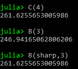
This results in the names getting spaced out almost the same as usual, but making better approximations to the important whole-number pitch ratios. For example, E in 19-TET is close to E in 12-TET, but a little flatter, closer to the just ratio.

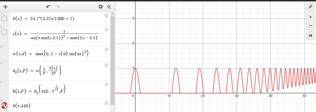
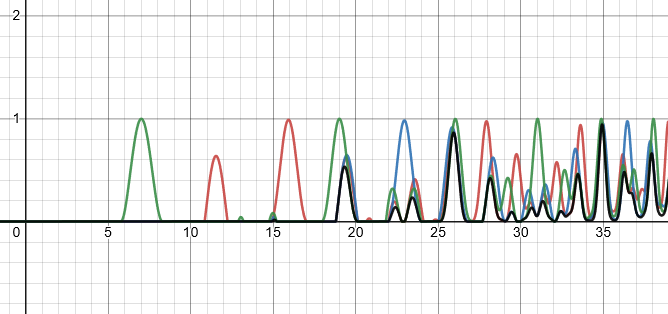
In using the visualizer, I was only able to see one thing, which wasn’t surprising: A# gets close to one of the overtones of a low C. More generally, the note 15/19ths above a root is it somewhat close to its “harmonic seventh,” an interval that 12-TET misses by a lot. Because that harmonic seventh is a feature of blues, I tried an experiment in boogie woogie. Making abundant use of that special interval in place of the typical dominant seventh, I made some formulaic boogie woogie music in Musescore, using a plugin to automatically adjust the pitches into 19-TET tuning.

I’m pleased with the result, though it is pretty harsh. I think the harshness is partly just because of the synthesized piano sound, partly because this tuning is alien to our 12-TET conditioned ears, and partly because I’m leaning on that seventh, which is a dissonant sound.

To round out our collection of important chord images, here are those of A minor as compared to the root A1. Making this made me appreciate how effective music theory already is at describing the phenomena we experience listening to music. Something important to notice here is that these chords here use all the same notes as the key of C major. But if a piece of music has implied to us a key of A minor, then hearing a G major chord (the bVII) we experience tension, pulling up up toward A. It’s as if G is interfering with the ghost of A in our heads.

And that same G is the V of C. If we look at our images (ignoring the diminished ii because that’s really harsh to listen to and not commonly used), we see that bVII is the one chord where one of the early overlaps lines up with the middle of an overtone of the base note. The images from the key of C major showed the same thing. In both cases it was a weak overlap, but it’s kind of like those notes are tightly squeezing at the base note. A difference is in the major key that occurs over one of the octaves of that base note, and here it occurs over one of the fifths.

Based on what I’ve seen, it seems like the amount of overlapping that occurs between the chord and the (possibly only implied, rather than physically present) base note prior to the chord’s own first significant internal overlap, correlates with the feeling of harmonic stability, whereas the amount of partial overlapping with the base note correlates with tension. And if an early chord-internal overlap occurs directly over an overtone of the base note, that creates a strong pull, an expectation of a cadence.

Overall, I am doubting the usefulness of the analysis I’ve done over the past few weeks, and the applicability to composition. I think the traditional tools of composition are well refined and didn’t really need the application of math when music is such a subjective and innate experience. That said, I will be keep the experience close at hand in my mind when composing music in the future. And next week I will still try and see what happens when I look at some other tuning system. I’m thinking to look at 19-tone equal temperament, because I heard this amazing song that uses it.

This week I updated my code so that it’s easier to use. Now one can refer to a specific note and get its frequency as easy as this:

And those numbers can be used as inputs to the visualizer, like this:

image = harmony_vis( nothing, B(flat, 4), D(5), F(5) );
save("B_flat_major.png", image)

image = harmony_vis( B(flat, 2), B(flat, 4), D(5), F(5) );
save("B_flat_major_over_B_flat_base_note.png", image)

That is also an example of how the function can be used to create those images of either three-note or four-note chords. If the first input is nothing (that’s a Julia object that represents nothing or no data, equivalent to Python’s None), then the visualizer will produce a two-rowed picture ( from the next three inputs. Otherwise, the first input will be used as the root note for a four-rowed picture. In either case, the three inputs after the first will be coloured red, green, and blue, respectively.

Here is a link to my Julia code.

Because this system made it clear what notes I was using, I realized some of the images from last week were using notes higher or lower than I had said, and many were labelled wrong in the gallery. I have since fixed those.

As well as four-note chords, I noticed this visualization scheme can be used to look at functional harmony, relating some three-note chord back to a “tonal center.” In the following gallery you can see how the main six diatonic chords in the key of C overlap with the harmonic series of C2. I have used inversions of the chords to keep them within a close pitch-range of one another. Also, I am assuming from prior work that, in a major key, what we hear as the tonal center is the note two octaves below the root of the I (one) chord. Conventionally because of the phenomenon of “octave equivalence,” we would just say that the tonal center is C. However, I am theorizing that the particular note is significant, that higher and lower ‘C’s are harmonically close to the tonal center, but distinct from it.

A nice thing about this collection is it shows all of the close-position inversions of major and minor chords. For next week I will keep looking for patterns in here, and focus on this functional harmony. Questions: Can this show us how a major key works? What about a minor key? What might this say about “borrowed chords?”

Also, I have noticed that this analysis can be easily generalized to notes outside the normal tuning (microtonal notes). So I will like to try using it to find nice-sounding microtonal harmonies, make a composition, and create some audio for that.

Full gallery here

Okay folks, this week the pictures are more colourful, and we can see all of pianospace. The left side is A_0, the bottom of a typical piano, and the right goes past the piano’s range and on to the upper limit of human hearing. Now that the overtone bands are properly smearing out, I should point out that they decrease in volume the higher up they are from the root. So to be totally accurate, we might need to lower the brightness toward the right, but the images are easier to read this way, and anyway, the particular way that a given series fades out depends on the timbre of the instrument producing it.

For these 3-note images, the top half shows all the harmonics while the bottom half shows just the parts that overlap with one another. Here’s another:

If you want to take a really good look you’ll have to open the image in a new tab. Now, musicians sometimes say that chords built from notes lower down get “muddy.” We’re seeing that just a little bit already, but let’s take a look at lower versions of C major.

Woah! Now the notes are clearly interfering with one another.

It’s a rainbow! Down here the notes are so “muddy” they completely smear together.

I said previously that I wanted to look at 4-note chord. I did find a way to do that.

These pictures are more complicated. Root note’s series is shown in white at the top, the other three notes are given in R, G, and B in the bottom-middle quarter and you can see them mixing there. In between are their overlaps with the root note, such as those first two thin bands of red and blue. And at the bottom are the overlaps of the coloured notes (non-root). Here’s one I especially like the sound of:

And here is a highly dissonant and also commonly used one:

One more interesting direction to go with this: adding more space between notes. You may remember from near the beginning of this inquiry I talked about a drop-2 minor chord, and that it should have a clear harmonic overlap early on, and that it sounds very consonant. Well here it is:

It seems at this point that we can state some patterns about these visualizations and how they relate to consonance and dissonance. The thin overlaps don’t seem to matter much; they’re probably not very perceptible. In highly consonant chords, the first significant overlap is a complete one. Whereas in highly dissonant chords, the first significant overlap is muddy. The above is an example where it’s kind of hard to say if those first two are significant, but then there is a very strong complete one. For another example of a clearly muddy one:

I’m excited to see if I can apply this technology to music composition.

This week I did some reading on Wikipedia, which I probably should have done sooner. I read about critical bandwidth, and also consonance and dissonance. The explanation I’m currently exploring is there, as well as several others including that one about long patterns I gave up on reading (although I am starting to think I didn’t give it enough credit) and the idea that the experience of dissonance is a response to rare or unusual sounds.

I took the formula for critical bandwidth and used it to build a new function for my visualizer. By the way, I have so far neglected to mention how I use Desmos. Many times in my life I have gone to Desmos with some mathematical question, and used it to tinker with functions and get a sense for them. In much the same way. Here is a reenactment of what it looked like to work on a new function:

That function in blue becomes the basis for the new model. What I ended up with was this:

Previously, the frequency bands of the harmonics shrunk down, so they would only have indicated overlap in the cases where it was very close. This time, we are using real frequencies. The y axis represents 440 Hz (standard A4), and the widths of the bands are given by that formula b(x), for which Wikipedia cites Glasberg and Moore. I can already tell that what this produces is going to produce more visually interesting. For example:

Hopefully it is also more useful and accurate in terms of how we hear. This week I hope to make some of those colour-gradient visualizations with this new model, and maybe figure out four-note chords. I imagine that I can continue to use just three colours, by ignoring the chord’s fifth, or using the same colour for it as for the root. Or maybe there is some method of combining four colours in a way that is still visually understandable.